Dirichlet Series
Motivation
Given a positive integer , what is the number of its divisors? This problem appears constantly in coding challenges. Write this number of divisors into a condense form
and let us also define this as a function in Julia with Primes.jl and plot the first values with CairoMakie.jl
using Primes
using CairoMakie

function d(n)
    prime_factors = factor(n)
    count = 1
    for (_, e) in prime_factors
        count *= (e + 1)
    end
    count
end

N = 100
ns = 1:N

fig = Figure()
ax = Axis(fig[1, 1],
    xlabel = L"n",
    ylabel = L"d(n)",
    xlabelsize = 20,
    ylabelsize = 20,
    title = "Number of divisors",
    titlesize = 24)

stem!(ax, ns, d.(ns); label=L"$d(n)$")

axislegend(ax;
    position = :lt,
    framevisible = true,
    labelsize = 20)

save(joinpath(@OUTPUT, "divisor_count.svg"), fig)
Seems quite random, however in this article we will discuss the following striking asymptoticity obtained by Dirichlet in 1849
as plotted
using CairoMakie

N = 100
ns = 1:N

function sumd(x)
    sum([d(n) for n in 1:floor(x)])
end

function xlog(x)
    x * log(x)
end

fig = Figure()
ax = Axis(fig[1, 1],
    xlabel = L"x",
    ylabel = L"\sum_{n \leq x} d(n)",
    xlabelsize = 20,
    ylabelsize = 20,
    title = "Asymtote",
    titlesize = 24)

stem!(ax, ns, sumd.(ns); label=L"$\sum_{n \leq x}d(n)$")
lines!(ax, ns, xlog.(ns); color=:red, label=L"$x \log x$")

axislegend(ax;
    position = :lt,
    framevisible = true,
    labelsize = 20,
    rowgap = 4)

save(joinpath(@OUTPUT, "asymtote.svg"), fig)
As shown above, the asymptotic formula is already evident for .
The correct way to study is through its Dirichlet series . I will present two reasons to introduce Dirichlet series: they capture the algebraic structure behind , and their poles and zeros reflects the behavior of as . This topic will motivate the study of analytic number theory.
Arithmetic Functions and Dirichlet Series
Let us extract the obvious information from the definition : it is a function defined on , and the sum is over divisors. This abstracts into the following definition.
Definition. The commutative ring of arithmetic functions is the set of functions
equipped with pointwise addition and multiplication given by convolution
The function
serves as unity.
For every arithmetic function there is an associated Dirichlet series . For now just ignore the convergence issue and consider this as a foraml series. The ring of formall Dirichlet series is nothing but , the complete monoid algebra of the multiplicative monoid . Our association defines a ring isomorphism
this would be clear once we notice that for the function
there is
Remark. Mapping to for each prime gives an isomorphism
where the right-hand side is the formal power series ring of independent variables indexed by prime numbers.
Now consider the constant function , we immediately check that , which means . This is better known as the Riemann function, the central object of analytic number theory. We will study the very basics of , then comes for free. But that will not be helpful unless we understand how can be used to study .
Perron's Formula
If the Dirichlet series converges absolutely at some , then convergence is guaranteed at every point to the right of . If we define
the Dirichlet series will converge as long as .
Assume and apply Abel's summation formula, we have
where . Absolute convergence is necessary since we need to interchange summation and integral.
After a change of variable , we see that is the Laplace transform of :
Apply the inverse Laplace transform and we get
where is any real number larger than . The left-hand side is often written as , the only difference from the usual is that when is an integer, the last term is replaced by . The above equality is called Perron's formula.
Contour Shifting
The Perron formula is exact, but it gives no information unless we can find the dominant terms. The idea is to shift the integral contour left to get a smaller integral, while the singularities crossed should contribute to the dominant terms.
Take for example, in this case is obvious, so we expect to obtain the same result from Dirichlet series . The series
converges for , and has a pole at . But what is to the left of this pole? The hope is to find a meromorphic function extending so that we can define on the points to the left of . This is called a meromorphic continuation. It turns out that has a meromorphic continuation to the entired complex plane But for our purpose, we just need to extend a little bit left, and the treatment is much easier.
Consider the alternating sum
which converges for (uniformly in compact subsets). The trick is
and therefore
for . The possible poles are from the zeros of , i.e. . Only is a pole and to show this we consider another function
which gives a different expression
Now the possible poles are of the form . Now that , the quotient cannot be a rational number, so is the only pole. We may plot the function as follows, the color reflects argument, and brightness reflects absolute value.
using CairoMakie, SpecialFunctions, Colors

# the domain
σs = range(0, 2, length=200)    # real part
ts = range(-1, 1, length=200)  # imaginary part

# evaluate ζ on the grid
Z = [zeta(σ + im*t) for σ in σs, t in ts]

# color each point by hue (arg) and lightness (|ζ|)
function domain_color(z)
    h = (angle(z) / (2π) + 1) % 1        # hue from arg, in [0,1)
    m = abs(z)
    # smoothly map magnitude to lightness: log scale, capped
    l = 0.5 + 0.5 * (2/π) * atan(log(m + 1e-10))
    return HSL(h * 360, 0.85, clamp(l, 0.1, 0.9))
end

img = domain_color.(Z)

fig = Figure(size=(400, 400))
ax = Axis(fig[1, 1],
    xlabel = L"\sigma",
    ylabel = L"t",
    title  = L"\zeta(\sigma + it)",
    aspect = DataAspect()
)

image!(ax, (0, 2), (-1, 1), img; interpolate=false)

save(joinpath(@OUTPUT, "zeta_domain_coloring.png"), fig)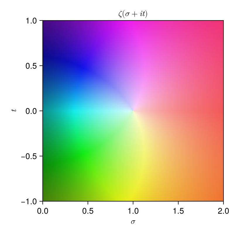
References
T. M. Apostol, Introduction to Analytic Number Theory, Undergraduate Texts in Mathematics, Springer, New York, 1976. DOI: 10.1007/978-1-4757-5579-4.
C. Sorensen, From Classical L-Functions to Modern Reciprocity Laws, Graduate Texts in Mathematics 307, Springer, Cham, 2025. DOI: 10.1007/978-3-032-03035-1.